ggplotly(getSSB(NS_sim))Pre-announcing mizer 3.0
mizer 3.0 brings new biological realism, improved numerics, a richer interactive analysis experience, and a composable extension framework
We are thrilled to pre-announce the release of mizer 3.0, the most significant update to the mizer R package since version 2.0. This release brings new biological realism, improved numerics, a richer interactive analysis experience, and a composable extension framework — all while remaining backwards compatible with your existing models.
We would love to get your feedback on the new version before we release it on CRAN, probably next week. So, if you can, install it from GitHub now:
pak("sizespectrum/mizer")We welcome bug reports and feature requests on GitHub.
We thank everyone in the mizer community who contributed ideas, and feedback that shaped this new mizer version. Claude, Codex and Gemini were very helpful in writing the code and documentation. Claude wrote this blog post.
Individual variability in growth: diffusion in the size spectrum
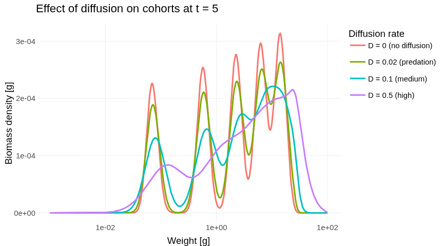
The headline addition in mizer 3.0 is a diffusion term in the McKendrick–von Foerster equation. Until now, mizer’s size-spectrum model treated growth as a purely advective process: every individual of a given species and size grows at the same rate. In reality, individuals of the same age and species vary considerably in size, and that spread in body size has measurable ecological consequences — for predation, reproduction, and the shape of the size spectrum itself.
The new diffusion term captures this individual variability as a spreading (or “diffusion”) of the abundance distribution along the size axis. Two sources of diffusion are now available:
-
External diffusion (
D_extspecies parameter, set viasetExtDiffusion()): a power-law diffusion rate you specify directly, representing any source of individual growth variability. -
Predation-induced diffusion (
use_predation_diffusion = TRUE): derived automatically from the jump-growth interpretation of predation, where consuming a prey item causes a discrete jump in body size rather than smooth growth.
The total diffusion rate at every body size is returned by the new getDiffusion() function, and the full flux of individuals (advective + diffusive) is available from getFlux(). The steady-state solution and project() both account for diffusion correctly, including at the recruitment boundary.
A new vignettes Cohort dynamics and diffusion demonstrates the effect of diffusion in a simple example.
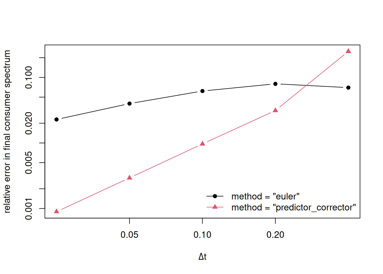
A second-order numerical scheme
project(), projectToSteady(), and steady() now accept a method argument. The default "euler" method is unchanged from previous versions. The new "predictor_corrector" option implements a second-order predictor–corrector scheme that delivers substantially better accuracy for the same time step, making it the recommended choice for demanding applications.
Simulation settings are now recorded in every MizerSim object via the new sim_params slot (accessible with getSimParams()), so you always know which method and time step produced a given result. When continuing a simulation from a MizerSim object, project() automatically uses the stored settings.
A new vignette on The Numerical Scheme used in Mizer describes the details of the numerical schemes.
Rich, interactive return values
One of the most user-visible changes in mizer 3.0 is that the arrays returned by mizer’s getter functions are no longer plain matrices — they carry metadata and come with built-in plot(), ggplotly(), print(), summary(), and as.data.frame() methods.
So to get, for example, a plot of the spawning stock biomass, you simply need
Three new S3 classes cover all the main cases:
| Class | Returned by | Shape |
|---|---|---|
ArraySpeciesBySize |
getEncounter(), getFeedingLevel(), getExtMort(), … |
species × size |
ArrayTimeBySpecies |
getBiomass(), getSSB(), getYield(), getN() on a MizerSim
|
time × species |
ArrayTimeBySpeciesBySize |
getFeedingLevel(), getPredMort(), getMort(), … on a MizerSim
|
time × species × size |
Each object carries a human-readable value_name and units attribute so that plot() can produce a labelled graph immediately, without requiring any manual axis annotation. ggplotly() wrappers convert every ggplot2 output into a fully interactive plotly figure with a single call.
For ArrayTimeBySpeciesBySize objects, an animate() method produces a smooth animation of the evolving size spectrum, supporting axis limits, interpolation, and background species. So if you want to see how the size-dependent mortality in the North Sea model has changed over the years you can simply do:
animate(getMort(NS_sim), wlim = c(10, NA))The addPlot() generic lets you overlay additional quantities on an existing figure, and the new plot2() and plotRelative() generics make it straightforward to compare two model states side by side.
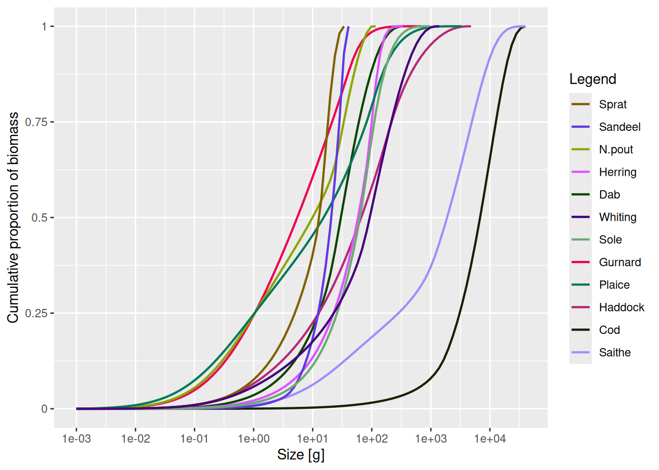
New cumulative distribution functions are also available: plotCDF() and plotCDF2() show the cumulative abundance or biomass distribution across sizes — a quick way to see how a fishery or environmental change reshapes the community size structure.
Composable extension chains
Mizer has long supported custom rate functions and ecosystem components. Version 3.0 introduces a composable extension chain that makes it possible to stack multiple independent extensions on a single model without them interfering with each other.
Extensions register themselves via registerExtension() and can define S3 methods for any of the projection hooks — projectEncounter(), projectFeedingLevel(), projectPredMort(), projectRDI(), and so on. Models without active extensions continue to use the original mizerRates() pipeline at full speed with no per-time-step overhead.
saveParams() and readParams() now preserve the extension chain, and new saveSim() and readSim() helpers do the same for simulation objects. This means shared models load correctly on any machine where the extension packages are installed, with pak invoked automatically to fetch missing dependencies.
Three new vignettes support extension authors and users:
-
Extending mizer — when to use
setRateFunction(),setComponent(), andcustomFunction(); required function signatures; worked examples - Using extension packages — a user-facing guide to loading and running extension-based models
- Creating a mizer extension package — a step-by-step guide for extension authors
New species parameters for external rates
A mizer model does not need to model all ecosystem components explicitly. So some part of mortality, prey encounter and diffusion rates comes from external sources. Three new species parameters give you control over rates that originate outside the explicitly modelled community:
-
z_extandd— add an allometric term to external mortality:mu_ext(w) = z0 + z_ext * w^d. Useful for representing predation by species not included in the model. -
E_ext— coefficient of an external allometric encounter ratew, set viasetExtEncounter(). Allows food subsidies from outside the model. -
D_ext— coefficient of an external allometric diffusion rate, as described above.
All three default to zero, so existing models are unaffected.
Other highlights
getTrophicLevel() calculates the trophic level of individuals at every body size, accounting for ontogenetic diet shifts by integrating over each individual’s growth trajectory. getMeanTrophicLevel() returns the consumption-weighted mean trophic level per species.
ggplotly(getTrophicLevel(NS_params))expandSizeGrid() extends the size grid of a MizerParams object to a new minimum and/or maximum size while preserving all existing species data. This is for example used by addSpecies() when you add a new species to an existing model that grows to sizes larger than previously includes species.
Verbosity control: an info_level argument has been added to projectToSteady(), steady(), setParams(), addSpecies(), newCommunityParams(), newTraitParams(), and the matchBiomasses()/matchNumbers()/matchYields() family. Set info_level = 0 to run these functions silently in pipelines or automated scripts.
compareParams() output has been reformatted for readability, with each differing slot shown as a separate block and per-species max differences reported for array slots.
A new cheatsheet vignette — Analysis and Plotting — provides a compact quick-reference for all functions that access simulation arrays, compute summaries, calculate indicators, and create plots.
For more changes see the Changelog.
Upgrading
mizer 3.0 introduces a few breaking changes:
The names of the dimnames of the arrays returned by
getMort(),getPredRate()are nowspandwto be in line with other functions likegetFMort().Functions that return arrays of the form (species x size), (time x species) or (time x species x size) now return them with extra attributes and an S3 class of
ArraySpeciesBySize,ArrayTimeBySpeciesorArrayTimeBySpeciesBySize. While this does not change their old behaviour, the differences will be flagged by functions likeis.identical()and such.plotDiet()no longer accepts atime_rangeargument.
Existing MizerParams and MizerSim objects are upgraded automatically when loaded with readParams() or readSim().