remotes::install_github("sizespectrum/mizerExperimental")
library(mizerExperimental)A 5-step recipe for tuning the model steady state
Getting a steady state for your mizer model that agrees with observations is in principle a hard chicken and egg problem. I present the trick that makes it surprisingly easy, with a 5-step recipe. I’ll save tips on what to do when the recipe fails for later blog posts.
What we want to do
In this blog post we will describe stage 2 of the process of building a mizer model. The stages are:
Collect information about the important species in your ecosystem and how they are fished. This includes physiological parameters for the species as they might be found on fishbase, but also information about how abundant the species are and how they are being fished.
Create a mizer model that in its steady state reproduces the time-averaged observed state of your fish community. Of course your real system never is in a perfect steady state. It is continuously changing. There is much fluctuation from year to year. We will however assume that if we average observations over a number of years we obtain something that is close to the steady state. Without some such assumption it would be impossible for us to get started.
Tune the model parameters further to also reproduce time-series observations that capture some of the system’s sensitivity to perturbations, like changes in fishing pressure.
This blog post is only about the second stage. We will present a 5 step recipe for that stage. When the recipe works, it will only take a couple of minutes! So I hope you will try the recipe for your own model. Of course in practice there are all kinds of things that can (and will) go wrong. So I hope this blog post will lead to some exchange of experiences with the recipe.
The recipe is based on an important trick. I call it the constant reproduction trick. The trick is obvious once you see it, but I must admit that I struggled for a long time with mizer model building until I stumbled upon the trick.
Example we will use
To make this concrete, we will consider a model for the North Sea involving 12 species. We will short-circuit stage 1 of the model-building process by basing our example on the North Sea species parameter data frame NS_species_params that comes with mizer.
Some of the functions we will be using are still in active development in the mizerExperimental package. Therefore we will always want to make sure we are loading the latest version of the package with
This blog post was compiled with mizer version 2.5.4.9011 and mizerExperimental version 2.5.3.9000
Here is the species parameter data frame that we will be using:
# Here is how I obtained the example species_params:
species_params <- NS_species_params
species_params$R_max <- NULL
species_params$a <- c(0.007, 0.001, 0.009, 0.002, 0.010, 0.006, 0.008, 0.004,
                         0.007, 0.005, 0.005, 0.007)
species_params$b <- c(3.014, 3.320, 2.941, 3.429, 2.986, 3.080, 3.019, 3.198,
                         3.101, 3.160, 3.173, 3.075)

years <- getTimes(NS_sim) >= 1990 & getTimes(NS_sim) <= 2010
# Average biomass over those 21 years
bm_hist <- getBiomass(NS_sim)[years, ]
species_params$biomass_observed <-  colSums(bm_hist) / 21

library(knitr)
kable(species_params, row.names = FALSE)| species | w_max | w_mat | beta | sigma | k_vb | w_inf | a | b | biomass_observed |
|---|---|---|---|---|---|---|---|---|---|
| Sprat | 33.0 | 13 | 51076 | 0.8 | 0.681 | 33.0 | 0.007 | 3.014 | 3.325300e+10 |
| Sandeel | 36.0 | 4 | 398849 | 1.9 | 1.000 | 36.0 | 0.001 | 3.320 | 1.115636e+12 |
| N.pout | 100.0 | 23 | 22 | 1.5 | 0.849 | 100.0 | 0.009 | 2.941 | 3.047268e+11 |
| Herring | 334.0 | 99 | 280540 | 3.2 | 0.606 | 334.0 | 0.002 | 3.429 | 4.286172e+11 |
| Dab | 324.0 | 21 | 191 | 1.9 | 0.536 | 324.0 | 0.010 | 2.986 | 1.723425e+10 |
| Whiting | 1192.0 | 75 | 22 | 1.5 | 0.323 | 1192.0 | 0.006 | 3.080 | 2.299098e+11 |
| Sole | 866.0 | 78 | 381 | 1.9 | 0.284 | 866.0 | 0.008 | 3.019 | 1.078201e+11 |
| Gurnard | 668.0 | 39 | 283 | 1.8 | 0.266 | 668.0 | 0.004 | 3.198 | 1.277013e+11 |
| Plaice | 2976.0 | 105 | 113 | 1.6 | 0.122 | 2976.0 | 0.007 | 3.101 | 2.197107e+12 |
| Haddock | 4316.5 | 165 | 558 | 2.1 | 0.271 | 4316.5 | 0.005 | 3.160 | 6.953041e+11 |
| Cod | 39851.3 | 1606 | 66 | 1.3 | 0.216 | 39851.3 | 0.005 | 3.173 | 3.054369e+11 |
| Saithe | 39658.6 | 1076 | 40 | 1.1 | 0.175 | 39658.6 | 0.007 | 3.075 | 8.099535e+11 |
For each species we are specifying its name and some parameters characteristic of the species: its asymptotic size w_inf and maturity size w_mat, the parameters beta and sigma for its feeding kernel (we are using the default lognormal kernel for all species), the von Bertalanffy growth parameter k_vb and the parameters a and b in the allometric length-weight relationship \(w = a l^b\).
In addition, we also specify information that is specific to our ecosystem, namely the average abundance of each species, in the biomass_observed column. This is measured in grams. Because for the purpose of this blog post it is not important, we did not bother to look up real biomass estimates but instead we simply used the average over the years 1990 to 2010 in the simulated data in the NS_sim object included in the mizer package. You are invited to re-run the analysis with proper data.
The observed system is being fished. We need to give mizer information about how it is being fished. We do this via the gear_params data frame.
# Average fishing mortality
f_location <- system.file("extdata", "NS_f_history.csv", package = "mizer")
f_history <- as(read.csv(f_location, row.names = 1), "matrix")[years, ]
f <- colSums(f_history) / 12

gear_params <-
    data.frame(gear = "All",
               species = NS_species_params$species,
               sel_func = "sigmoid_length",
               l25 =  c(7.6, 9.8, 8.7, 10.1, 11.5, 19.8, 16.4, 19.8, 11.5,
                        19.1, 13.2, 35.3),
               l50 = c(8.1, 11.8, 12.2, 20.8, 17.0, 29.0, 25.8, 29.0, 17.0,
                       24.3, 22.9, 43.6),
               catchability = f)

kable(gear_params, row.names = FALSE)| gear | species | sel_func | l25 | l50 | catchability |
|---|---|---|---|---|---|
| All | Sprat | sigmoid_length | 7.6 | 8.1 | 1.3763157 |
| All | Sandeel | sigmoid_length | 9.8 | 11.8 | 1.3331618 |
| All | N.pout | sigmoid_length | 8.7 | 12.2 | 1.3763157 |
| All | Herring | sigmoid_length | 10.1 | 20.8 | 0.8626210 |
| All | Dab | sigmoid_length | 11.5 | 17.0 | 0.2059334 |
| All | Whiting | sigmoid_length | 19.8 | 29.0 | 1.3429086 |
| All | Sole | sigmoid_length | 16.4 | 25.8 | 1.4424019 |
| All | Gurnard | sigmoid_length | 19.8 | 29.0 | 0.1342909 |
| All | Plaice | sigmoid_length | 11.5 | 17.0 | 1.0296672 |
| All | Haddock | sigmoid_length | 19.1 | 24.3 | 1.1690897 |
| All | Cod | sigmoid_length | 13.2 | 22.9 | 1.6476887 |
| All | Saithe | sigmoid_length | 35.3 | 43.6 | 0.9744912 |
We are setting up a single gear that we call “All” which catches all species. For each species we set up the selectivity curve of the gear as a sigmoid curve with given l25 and l50 parameters. Finally we set the catchability of each species to the observed fishing mortality, averaged over the years 1990 to 2010. We will then set the fishing effort to 1, because in mizer the fishing mortality is the product of effort, catchability and selectivity.
Our task now is to create a mizer model that describes species with the above characteristics and that has a steady state with the observed biomasses under the given fishing pressure.
Why it is a hard problem
We have a chicken and egg problem. The equilibrium abundance and size distributions of the fish are determined by their size-dependent growth and death rates. These rates in turn are determined by the abundance and size distribution of their prey and their predators. So we can’t determine the size distributions before we have determined the rates and we can’t determine the rates before we have determined the size distributions.
Because every species is a both prey and predator of fish of various species and sizes during their life, this is a highly coupled non-linear problem. If for example we use 100 size bins and 12 species, plus a resource spectrum, then we would have far over a thousand coupled nonlinear equations to solve simultaneously. That is not practical.
Rather than solving the equilibrium equations, another way to find a steady state is to simply evolve the time dynamics until the system settles down to a steady state. The problem with this approach is that the coexistence steady state of a size spectrum model has a very small region of attraction, so unless one starts with an initial state that is already very close to that coexistence steady state one will end up with extinctions.
The reason is a feedback loop: as the spawning stock biomass of a species grows, also its reproduction rate grows, leading to further growth of the spawning stock biomass and so on. Similarly as the spawning stock of another species declines, so does its reproduction rate, leading to further decline. In spite of moderating non-linear effects in the model, the general outcome is extinctions.
We can see the phenomenon in our North Sea example. If we simply run the dynamics, starting with the initial state set up by newMultispeciesParams(), first Sprat goes extinct, and Herring follows soon after. Just click the play button on the animation below.
params <- newMultispeciesParams(species_params = species_params,
                                gear_params = gear_params,
                                initial_effort = 1)
Because you have n != p, the default value for `h` is not very good.
Because the age at maturity is not known, I need to fall back to using
von Bertalanffy parameters, where available, and this is not reliable.
No ks column so calculating from critical feeding level.
Using z0 = z0pre * w_max ^ z0exp for missing z0 values.
Using f0, h, lambda, kappa and the predation kernel to calculate gamma.sim <- project(params, t_max = 12)
animateSpectra(sim, power = 2)The constant reproduction trick
So the trick is to cut the destabilising feedback loop by decoupling the reproductive rate from the spawning stock biomass. We do this by simply keeping the reproduction rate constant. The size spectrum model with constant reproduction turns out to be very stable and quickly approach a steady state, due to the smoothing effect of the feeding kernel. Once the steady state is found, we can simply adjust the reproductive efficiency of each species so that the steady state spawning stock produces the chosen reproduction rate. With that choice of the reproductive efficiency the steady state of the restricted dynamics is also the steady state of the full size spectrum model.
Here is the code that does that. Run the animation that it produces by clicking the play button.
params <- newMultispeciesParams(species_params = species_params,
                                gear_params = gear_params,
                                initial_effort = 1)
Because you have n != p, the default value for `h` is not very good.
Because the age at maturity is not known, I need to fall back to using
von Bertalanffy parameters, where available, and this is not reliable.
No ks column so calculating from critical feeding level.
Using z0 = z0pre * w_max ^ z0exp for missing z0 values.
Using f0, h, lambda, kappa and the predation kernel to calculate gamma.# Keep reproduction constant at the initial level
params@species_params$constant_reproduction <- getRDD(params)
params <- setReproduction(params, RDD = "constantRDD")
# Run the dynamics with this constant reproduction
sim <- project(params, t_max = 15)
animateSpectra(sim, power = 2)Mizer has a function called steady() that does the same as the above code, namely run to steady state with constant reproduction and then adjust the reproduction parameters, and then sets the resulting steady state as the initial state of the MizerParams object.
params <- newMultispeciesParams(species_params = species_params,
                                gear_params = gear_params,
                                initial_effort = 1)
Because you have n != p, the default value for `h` is not very good.
Because the age at maturity is not known, I need to fall back to using
von Bertalanffy parameters, where available, and this is not reliable.
No ks column so calculating from critical feeding level.
Using z0 = z0pre * w_max ^ z0exp for missing z0 values.
Using f0, h, lambda, kappa and the predation kernel to calculate gamma.params <- steady(params)Convergence was achieved in 18 years.plotlySpectra(params, power = 2)We now have a MizerParams object whose initial state is a steady state. Running a simulation starting with these initial conditions will show no change over time. For example the biomasses of all species will stay constant.
sim <- project(params, t_max = 5)
plotBiomass(sim)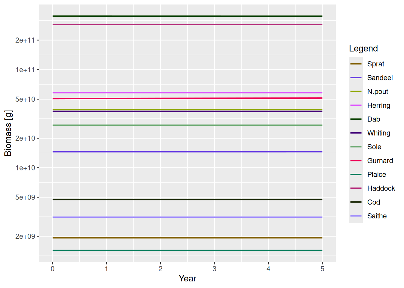
But how do these biomasses compare to our observed biomasses?
plotBiomassObservedVsModel(params, ratio = FALSE)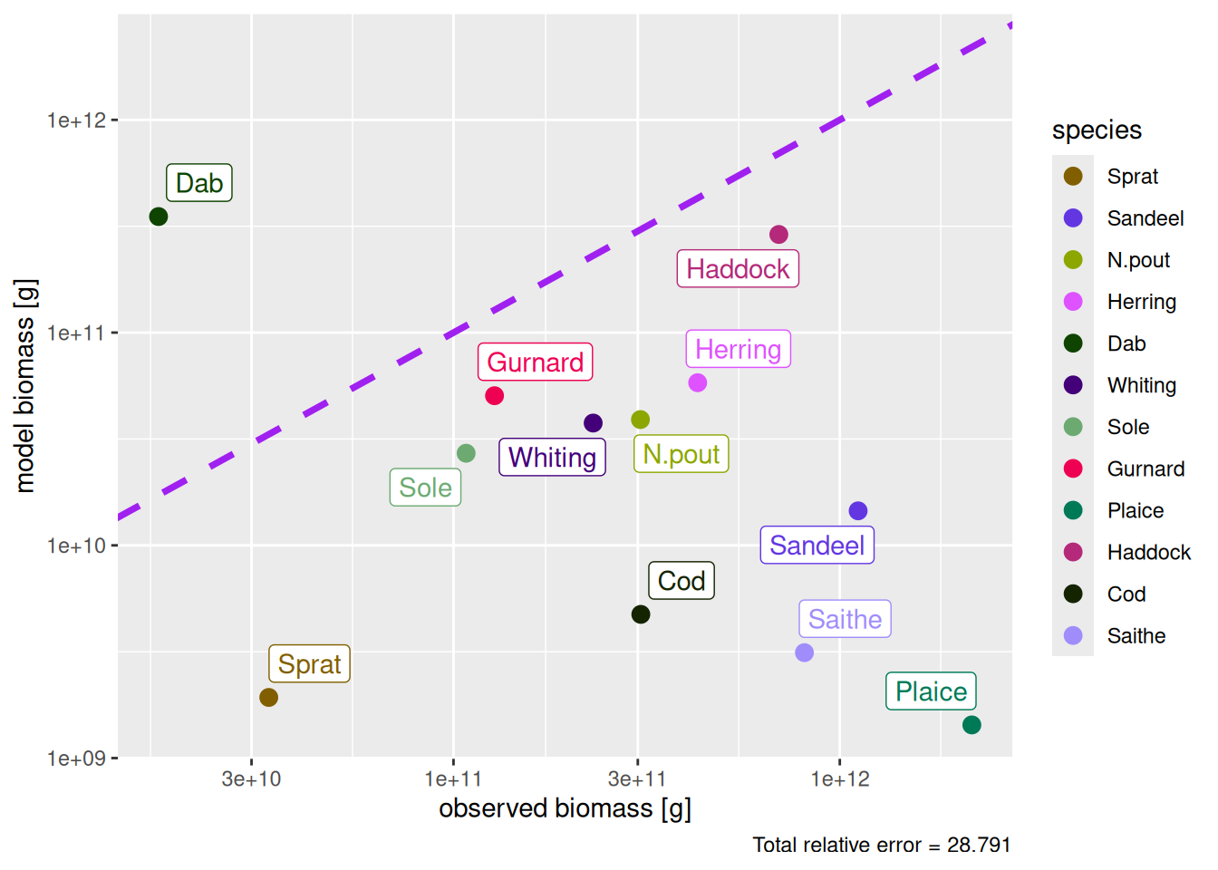
They don’t agree at all, but that is no surprise. It would actually have been quite a coincidence if they did agree, because the newMultispeciesParams() function did not know how big our ecosystem is. It did not know that we wanted the biomasses in the entire North Sea. So initially the scale is arbitrary. The dynamics of the model are obviously independent of the scale of the system. So we have the freedom to change that scale. The calibrateBiomass() function chooses the scale so that the total biomass in the model agrees with the total observed biomass.
params <- calibrateBiomass(params)
plotBiomassObservedVsModel(params, ratio = FALSE)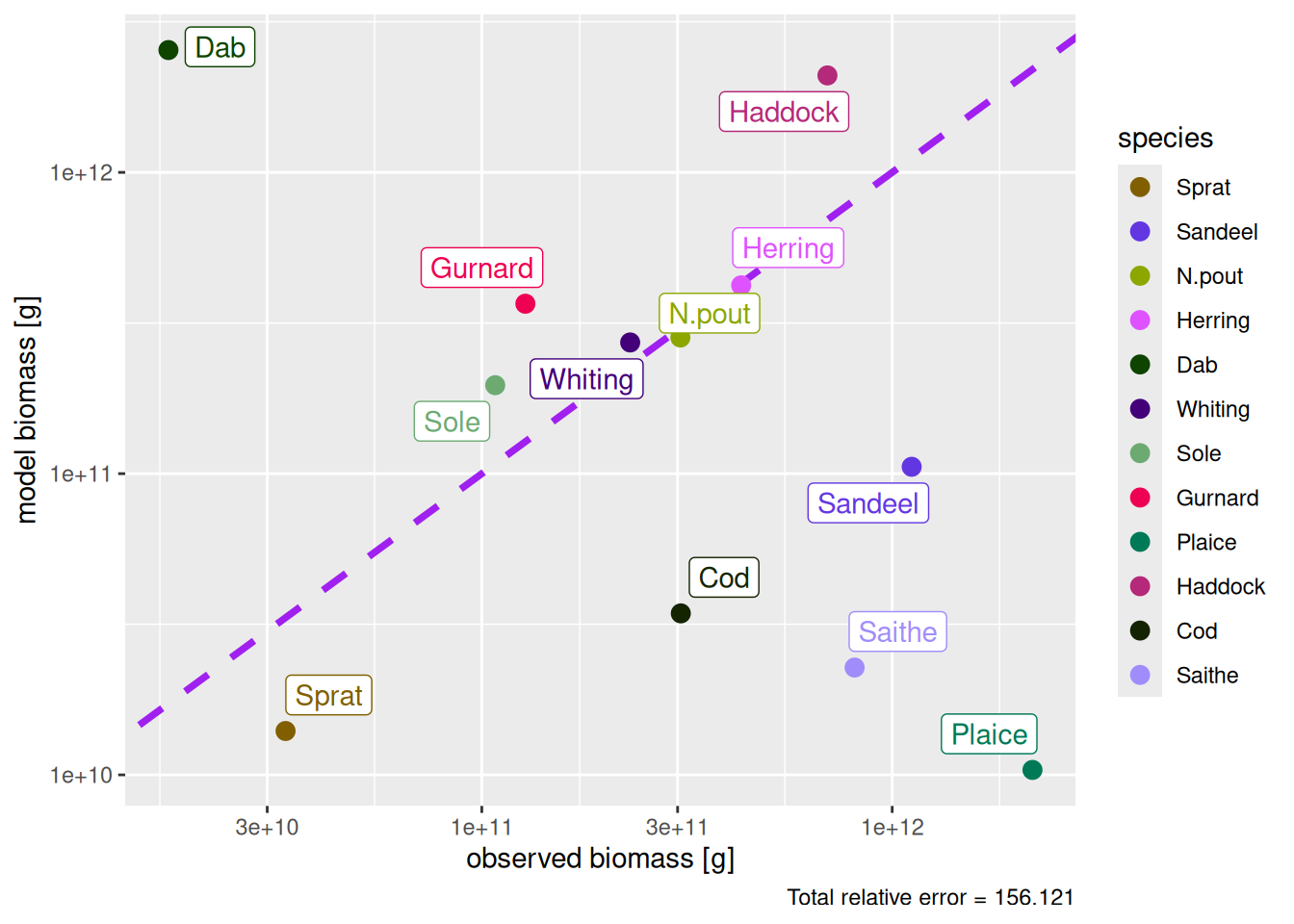
So now the total biomass is correct, but for some species the biomass in the model is too high, for others it is too low.
Actually, that the size spectrum is too low for Saithe and Cod and too high for Dab and Haddock might also be suspected from the fact that they are outliers in the size-spectrum plot above. We expect in a healthy ecosystem that the total spectrum roughly follows a power law, i.e., a straight line on the log-log plot. Those species currently spoil that.
So we want to lower the spectra of the species whose biomass is too high in the model and raise those of the species whose biomass is too low. This is what the matchBiomasses() function does.
params <- matchBiomasses(params)Warning in setBevertonHolt.MizerParams(params): For the following species `erepro` has been increased to the smallest possible value: erepro[Sprat] = 0.574; erepro[Sandeel] = 0.0125; erepro[Cod] = 7.94e-05; erepro[Saithe] = 1.28e-05plotlySpectra(params, power = 2, total = TRUE)In fact, it has raised and lowered the spectra by exactly the factor needed to get the model biomasses to match the observed biomasses.
plotBiomassObservedVsModel(params, ratio = FALSE)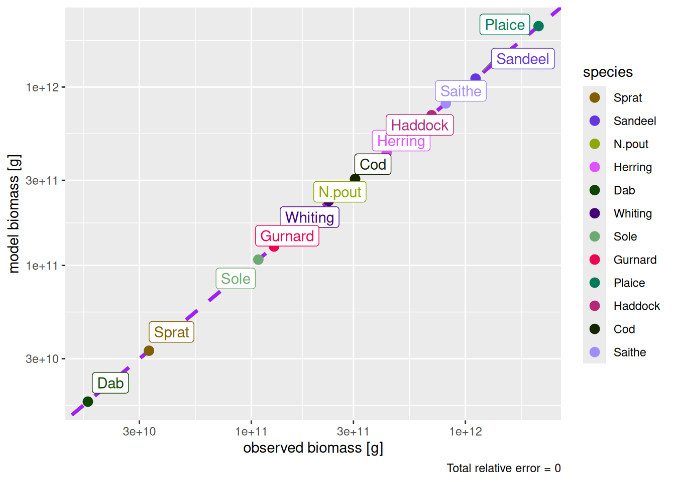
Of course this is not the end of the story, because just rescaling the size spectra by constants will not again produce a steady state. All species now experience a new prey distribution and a new predator distribution, so their growth and death rates have changed. We will have to again run the dynamics to steady state.
params <- steady(params)Convergence was achieved in 12 years.plotBiomassObservedVsModel(params, ratio = FALSE)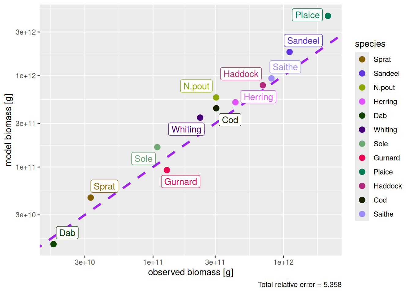
This has now spoiled the agreement between observed and model biomasses. But we can simply calibrate and match again and run to steady state again.
params <- params |> calibrateBiomass() |> matchBiomasses() |> steady()Warning in setBevertonHolt.MizerParams(params): For the following species `erepro` has been increased to the smallest possible value: erepro[Cod] = 3.65e-05; erepro[Saithe] = 8.51e-06Convergence was achieved in 10.5 years.plotBiomassObservedVsModel(params, ratio = FALSE)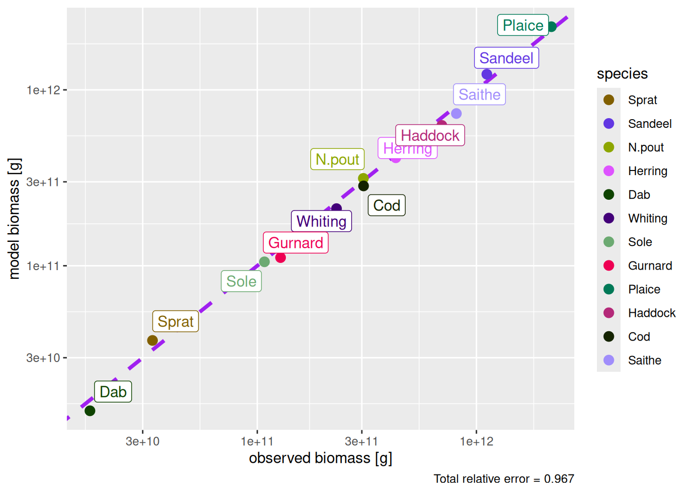
The discrepancies are now quite small. We could iterate to get them even smaller:
params <- params |> calibrateBiomass() |> matchBiomasses() |> steady() |>
    calibrateBiomass() |> matchBiomasses() |> steady()
Warning in setBevertonHolt.MizerParams(params): For the following species `erepro` has been increased to the smallest possible value: erepro[Cod] = 3.96e-05Convergence was achieved in 7.5 years.Convergence was achieved in 6 years.plotBiomassObservedVsModel(params, ratio = FALSE)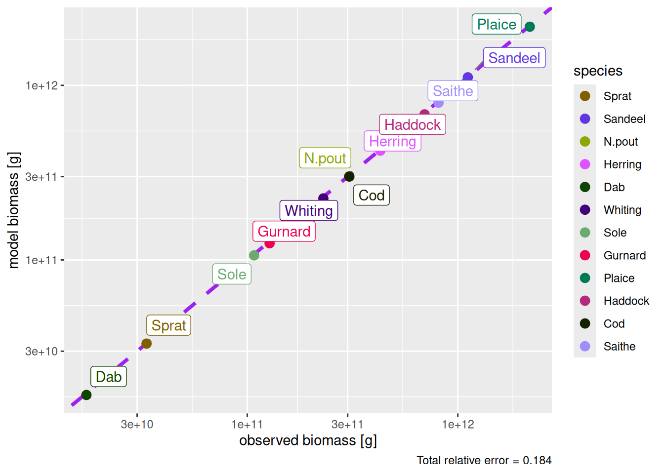
So here is the picture of the steady state that matches the observed biomasses:
plotlySpectra(params, power = 2)Actually, even the growth rates in the steady state match the von Bertalanffy growth curves pretty well:
plotGrowthCurves(params, species_panel = TRUE)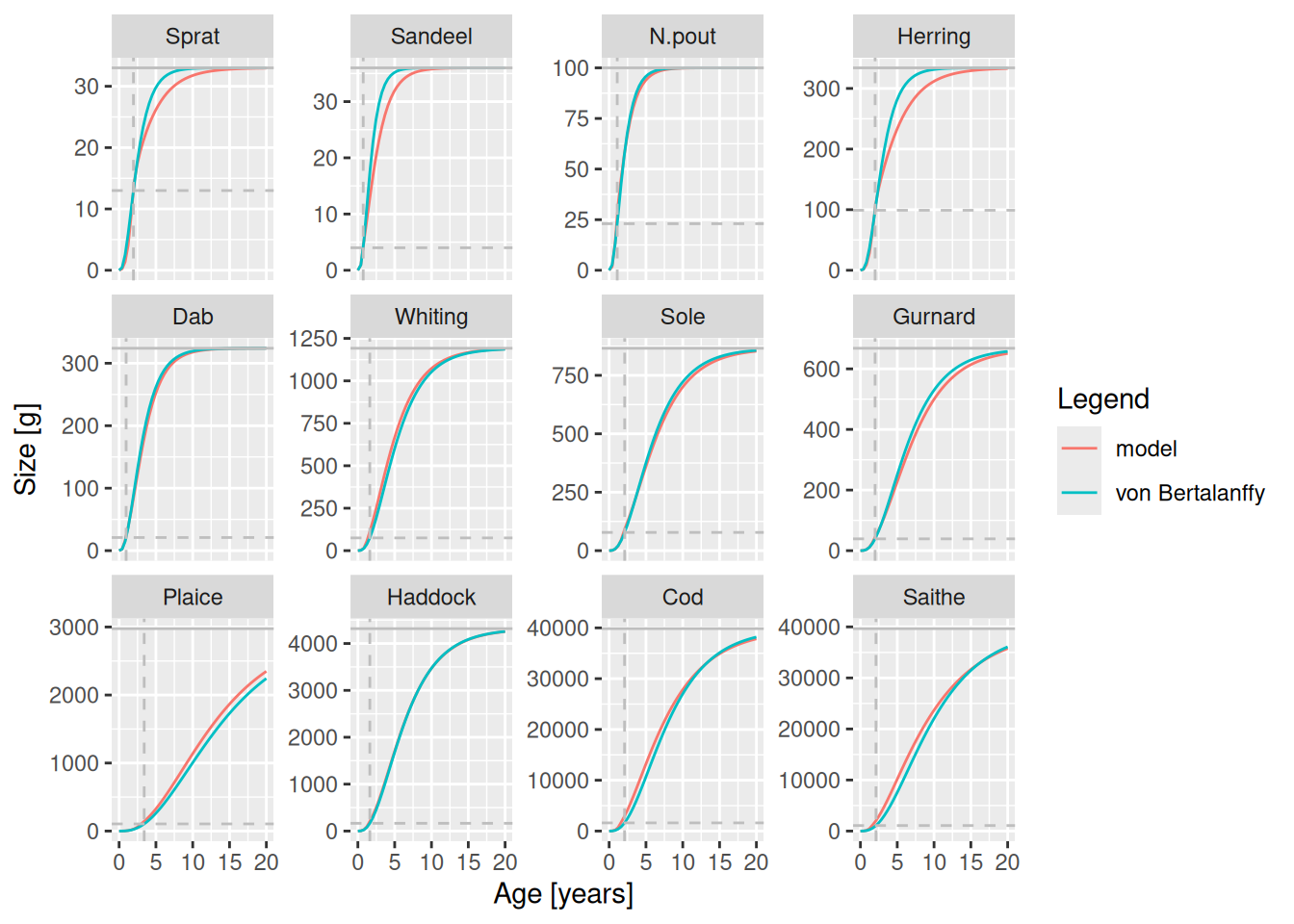
But this is a bit of a coincidence. Mizer has to choose values for the coefficient gamma of the ‘search volume’ for each species and for the coefficient ‘h’ of the maximum intake rate, both of which affect the growth rates. Because mizer has to choose them before it knows what the steady state prey distribution is for each species, it can not guarantee to choose them so as to give the correct growth rates in the steady state. You usually will have to retune them by hand. The mizerExperimental package provides a convenient shiny gadget that allows you to do that interactively, and I will talk about that in future blog posts.
Also remember that getting the steady state to agree with time-averaged observations is just the second stage in tuning a mizer model. Next you will want to tune the sensitivity to changes away from steady state. This will in particular involve tuning the density dependence in reproduction, among other things.
Summary of the recipe
We have seen how to proceed if you have your species parameters and gear parameters and also have averaged observed biomasses for each species that you want the steady state of your model to match:
Create a MizerParams object from your species parameters and gear parameters with
newMultispeciesParams().Find a coexistence steady state with
steady().Set the scale of the model to agree with the observed total biomass with
calibrateBiomass(). This does not spoil the steady state.Use
matchBiomass()to move the size spectra of the species up or down to match the observed biomasses. This will spoil the steady state.Go back to step 2 to again find the steady state. Iterate steps 2, 3 and 4 as often as you like to get the steady-state biomasses to agree as precisely with your observations as you like.
There are several interesting ways in which the above recipe can fail. I’ll blog about them in the future. But it will be more fun if you share your attempt at following the above recipe with your species parameters and your observed biomasses. Email me at gustav.delius@gmail.com. I can then use your example to explain what to do when problems arise.